Background #
A dataset was provided for a website that featured recipes on their homepage. Approximately 60% of the recipes featured led to “high traffic” on the website, driving new subscription sales. The following notebook explores the objectives of correctly predicting high traffic recipes 80% of the time.
1 cell collapsed:
import pandas as pd
import numpy as np
import matplotlib.pyplot as plt
import seaborn as sns
from scipy.stats import ks_2samp, pointbiserialr
1. Data Validation #
The data has 947 rows, 8 columns. I have validated all variables and I made several changes after validation: removed null values from nutritional value columns (calories, carbohydrate, sugar, and protein), and the target variable (high_traffic) was binary encoded to replace null values.
- recipe: 947 unique values without missing values, same as description. No cleaning needed.
- calories: numeric values as described, containing 52 missing values. Cleaning described in ‘Nutritional Value Cleaning’.
- carbohydrate: numeric values as described, containing 52 missing values. Cleaning described in ‘Nutritional Value Cleaning’.
- sugar: numeric values as described, containing 52 missing values. Cleaning described in ‘Nutritional Value Cleaning’.
- protein: numeric values as described, containing 52 missing values. Cleaning described in ‘Nutritional Value Cleaning’.
- category: 11 categories provided when only 10 specified in data dictionary. The discrepancy was due to ‘Chicken’ and ‘Chicken Breast’ both existing. The incorrect category was cleaned to the proper ‘Chicken’ category. Additionally the data type was updated categorical. There were no missing values.
- servings: Data provided was not imported as numeric as specified in data dictionary due to some values ending with ‘as a snack’. These ‘as a snack’ entries were already in the snack category. Data was cleaned to remove the ‘as a snack’ and then the data type was updated to integer as defined by data dictionary. There were no missing values.
- high_traffic: Verified contents marked as ‘High’ traffic as stated in data dictionary. Non-High traffic were indicated by missing values. As part of data cleaning and preprocessing this was binary encoded with 1 indicating high traffic and 0 as Non-High traffic. Additionally the data type was changed to integer. These changes were made to prepare the column for machine learning. After binary encoding there were no missing values and all values fell within a value of 0 or 1.
16 cells collapsed:
df = pd.read_csv('recipe_site_traffic_2212.csv')
df.info()
<class 'pandas.core.frame.DataFrame'>
RangeIndex: 947 entries, 0 to 946
Data columns (total 8 columns):
 #   Column        Non-Null Count  Dtype
---  ------        --------------  -----
 0   recipe        947 non-null    int64
 1   calories      895 non-null    float64
 2   carbohydrate  895 non-null    float64
 3   sugar         895 non-null    float64
 4   protein       895 non-null    float64
 5   category      947 non-null    object
 6   servings      947 non-null    object
 7   high_traffic  574 non-null    object
dtypes: float64(4), int64(1), object(3)
memory usage: 59.3+ KB
df.head()
| recipe | calories | carbohydrate | sugar | protein | category | servings | high_traffic | |
|---|---|---|---|---|---|---|---|---|
| 0 | 1 | NaN | NaN | NaN | NaN | Pork | 6 | High |
| 1 | 2 | 35.48 | 38.56 | 0.66 | 0.92 | Potato | 4 | High |
| 2 | 3 | 914.28 | 42.68 | 3.09 | 2.88 | Breakfast | 1 | NaN |
| 3 | 4 | 97.03 | 30.56 | 38.63 | 0.02 | Beverages | 4 | High |
| 4 | 5 | 27.05 | 1.85 | 0.80 | 0.53 | Beverages | 4 | NaN |
def validate_helper(df, col: str, unique_list:bool=True):
    """Prints basic info to help validate a column."""
    print(f'{col}:\nmissing values: {df[col].isna().sum()}\nunique values: {df[col].nunique()}')
    if unique_list:
        print(f'unique value list: {df[col].unique()}')
    print(df[col].describe())
# validate recipe
validate_helper(df, 'recipe', unique_list=False)
recipe_min = df['recipe'].min()
recipe_max = df['recipe'].max()
recipe_expected_sum = (recipe_max - recipe_min + 1) * (recipe_min + recipe_max) / 2
recipe_actual_sum = df['recipe'].sum()
if recipe_expected_sum == recipe_actual_sum:
    print("The 'recipe' column is a unique identifier.")
else:
    print("The 'recipe' column is NOT a unique identifier.")
recipe:
missing values: 0
unique values: 947
count    947.000000
mean     474.000000
std      273.519652
min        1.000000
25%      237.500000
50%      474.000000
75%      710.500000
max      947.000000
Name: recipe, dtype: float64
The 'recipe' column is a unique identifier.
# validate 'calories'
validate_helper(df, 'calories', unique_list=False)

# look at n/a values
df[df['calories'].isna()]
calories:
missing values: 52
unique values: 891
count     895.000000
mean      435.939196
std       453.020997
min         0.140000
25%       110.430000
50%       288.550000
75%       597.650000
max      3633.160000
Name: calories, dtype: float64
| recipe | calories | carbohydrate | sugar | protein | category | servings | high_traffic | |
|---|---|---|---|---|---|---|---|---|
| 0 | 1 | NaN | NaN | NaN | NaN | Pork | 6 | High |
| 23 | 24 | NaN | NaN | NaN | NaN | Meat | 2 | NaN |
| 48 | 49 | NaN | NaN | NaN | NaN | Chicken Breast | 4 | NaN |
| 82 | 83 | NaN | NaN | NaN | NaN | Meat | 4 | High |
| 89 | 90 | NaN | NaN | NaN | NaN | Pork | 6 | High |
| 116 | 117 | NaN | NaN | NaN | NaN | Chicken Breast | 6 | High |
| 121 | 122 | NaN | NaN | NaN | NaN | Dessert | 2 | High |
| 136 | 137 | NaN | NaN | NaN | NaN | One Dish Meal | 2 | High |
| 149 | 150 | NaN | NaN | NaN | NaN | Potato | 2 | High |
| 187 | 188 | NaN | NaN | NaN | NaN | Pork | 4 | High |
| 209 | 210 | NaN | NaN | NaN | NaN | Dessert | 2 | High |
| 212 | 213 | NaN | NaN | NaN | NaN | Dessert | 4 | High |
| 221 | 222 | NaN | NaN | NaN | NaN | Dessert | 1 | NaN |
| 249 | 250 | NaN | NaN | NaN | NaN | Chicken | 6 | NaN |
| 262 | 263 | NaN | NaN | NaN | NaN | Chicken | 4 | NaN |
| 278 | 279 | NaN | NaN | NaN | NaN | Lunch/Snacks | 4 | High |
| 280 | 281 | NaN | NaN | NaN | NaN | Meat | 1 | High |
| 297 | 298 | NaN | NaN | NaN | NaN | Lunch/Snacks | 6 | NaN |
| 326 | 327 | NaN | NaN | NaN | NaN | Potato | 4 | High |
| 351 | 352 | NaN | NaN | NaN | NaN | Potato | 4 | High |
| 354 | 355 | NaN | NaN | NaN | NaN | Pork | 4 | High |
| 372 | 373 | NaN | NaN | NaN | NaN | Vegetable | 2 | High |
| 376 | 377 | NaN | NaN | NaN | NaN | Pork | 6 | High |
| 388 | 389 | NaN | NaN | NaN | NaN | Lunch/Snacks | 4 | High |
| 405 | 406 | NaN | NaN | NaN | NaN | Vegetable | 4 | High |
| 427 | 428 | NaN | NaN | NaN | NaN | Vegetable | 4 | High |
| 455 | 456 | NaN | NaN | NaN | NaN | Pork | 6 | High |
| 530 | 531 | NaN | NaN | NaN | NaN | Vegetable | 1 | High |
| 534 | 535 | NaN | NaN | NaN | NaN | Chicken | 2 | High |
| 538 | 539 | NaN | NaN | NaN | NaN | Vegetable | 4 | High |
| 545 | 546 | NaN | NaN | NaN | NaN | Chicken Breast | 6 | High |
| 555 | 556 | NaN | NaN | NaN | NaN | Meat | 2 | NaN |
| 573 | 574 | NaN | NaN | NaN | NaN | Lunch/Snacks | 4 | NaN |
| 581 | 582 | NaN | NaN | NaN | NaN | Chicken | 1 | NaN |
| 608 | 609 | NaN | NaN | NaN | NaN | Chicken Breast | 4 | NaN |
| 674 | 675 | NaN | NaN | NaN | NaN | Pork | 4 | High |
| 683 | 684 | NaN | NaN | NaN | NaN | Potato | 1 | High |
| 711 | 712 | NaN | NaN | NaN | NaN | Lunch/Snacks | 4 | High |
| 712 | 713 | NaN | NaN | NaN | NaN | Pork | 6 | High |
| 749 | 750 | NaN | NaN | NaN | NaN | Dessert | 4 | High |
| 765 | 766 | NaN | NaN | NaN | NaN | Pork | 1 | High |
| 772 | 773 | NaN | NaN | NaN | NaN | One Dish Meal | 4 | NaN |
| 851 | 852 | NaN | NaN | NaN | NaN | Lunch/Snacks | 4 | High |
| 859 | 860 | NaN | NaN | NaN | NaN | One Dish Meal | 4 | NaN |
| 865 | 866 | NaN | NaN | NaN | NaN | Lunch/Snacks | 6 | High |
| 890 | 891 | NaN | NaN | NaN | NaN | Meat | 4 | High |
| 893 | 894 | NaN | NaN | NaN | NaN | One Dish Meal | 4 | NaN |
| 896 | 897 | NaN | NaN | NaN | NaN | Chicken | 6 | High |
| 911 | 912 | NaN | NaN | NaN | NaN | Dessert | 6 | High |
| 918 | 919 | NaN | NaN | NaN | NaN | Pork | 6 | High |
| 938 | 939 | NaN | NaN | NaN | NaN | Pork | 4 | High |
| 943 | 944 | NaN | NaN | NaN | NaN | Potato | 2 | High |
# validate 'carbohydrate'
validate_helper(df, 'carbohydrate', unique_list=False)
carbohydrate:
missing values: 52
unique values: 835
count    895.000000
mean      35.069676
std       43.949032
min        0.030000
25%        8.375000
50%       21.480000
75%       44.965000
max      530.420000
Name: carbohydrate, dtype: float64
# validate 'sugar'
validate_helper(df, 'sugar', unique_list=False)
sugar:
missing values: 52
unique values: 666
count    895.000000
mean       9.046547
std       14.679176
min        0.010000
25%        1.690000
50%        4.550000
75%        9.800000
max      148.750000
Name: sugar, dtype: float64
# validate 'protein'
validate_helper(df, 'protein', unique_list=False)
protein:
missing values: 52
unique values: 772
count    895.000000
mean      24.149296
std       36.369739
min        0.000000
25%        3.195000
50%       10.800000
75%       30.200000
max      363.360000
Name: protein, dtype: float64
# validate 'category'
validate_helper(df, 'category', unique_list=True)

# query 'chicken_breast' and 'chicken'
count_before = df[df['category'].isin(['Chicken Breast', 'Chicken'])].shape[0]
print("count before modification:", count_before)

# clean 'chicken_breast'
df.loc[df['category'] == 'Chicken Breast', 'category'] = 'Chicken'
count_after = df[df['category'] == 'Chicken'].shape[0]
print("count after modification:", count_after)

# update dtype to categorical.
df['category'] = df['category'].astype('category')
df['category'].dtype
category:
missing values: 0
unique values: 11
unique value list: ['Pork' 'Potato' 'Breakfast' 'Beverages' 'One Dish Meal' 'Chicken Breast'
 'Lunch/Snacks' 'Chicken' 'Vegetable' 'Meat' 'Dessert']
count           947
unique           11
top       Breakfast
freq            106
Name: category, dtype: object
count before modification: 172
count after modification: 172


CategoricalDtype(categories=['Beverages', 'Breakfast', 'Chicken', 'Dessert',
                  'Lunch/Snacks', 'Meat', 'One Dish Meal', 'Pork', 'Potato',
                  'Vegetable'],
, ordered=False)
# validate 'servings'
validate_helper(df, 'servings', unique_list=True)

# servings has object datatype and 6 unique values, suggesting one or more are formatted incorrectly
df['servings'].unique

if pd.api.types.is_string_dtype(df['servings']):
    df[df['servings'].isin(['4 as a snack', '6 as a snack'])]

    # clean 'as a snack'
    df['servings'] = df['servings'].str.replace(' as a snack', '', regex=False)

    # change dtype
    df['servings'] = df['servings'].astype(int)
servings:
missing values: 0
unique values: 6
unique value list: ['6' '4' '1' '2' '4 as a snack' '6 as a snack']
count     947
unique      6
top         4
freq      389
Name: servings, dtype: object
# validate high traffic
validate_helper(df,'high_traffic', unique_list=True)

# binary encode, replacing 'high' as 1, and missing values as 0.
df['high_traffic'] = df['high_traffic'].replace('High', 1).fillna(0)

# verify no more missing values
print(f"missing values remaining: {df['high_traffic'].isna().sum()}")

# change dtype to int, to prepare for machine learning
df['high_traffic'] = df['high_traffic'].astype(int)

# check unique values
print(f"new unique values: {df['high_traffic'].unique()}")
high_traffic:
missing values: 373
unique values: 1
unique value list: ['High' nan]
count      574
unique       1
top       High
freq       574
Name: high_traffic, dtype: object
missing values remaining: 0
new unique values: [1 0]
df.describe()
| recipe | calories | carbohydrate | sugar | protein | servings | high_traffic | |
|---|---|---|---|---|---|---|---|
| count | 947.000000 | 895.000000 | 895.000000 | 895.000000 | 895.000000 | 947.000000 | 947.000000 |
| mean | 474.000000 | 435.939196 | 35.069676 | 9.046547 | 24.149296 | 3.477297 | 0.606125 |
| std | 273.519652 | 453.020997 | 43.949032 | 14.679176 | 36.369739 | 1.732741 | 0.488866 |
| min | 1.000000 | 0.140000 | 0.030000 | 0.010000 | 0.000000 | 1.000000 | 0.000000 |
| 25% | 237.500000 | 110.430000 | 8.375000 | 1.690000 | 3.195000 | 2.000000 | 0.000000 |
| 50% | 474.000000 | 288.550000 | 21.480000 | 4.550000 | 10.800000 | 4.000000 | 1.000000 |
| 75% | 710.500000 | 597.650000 | 44.965000 | 9.800000 | 30.200000 | 4.000000 | 1.000000 |
| max | 947.000000 | 3633.160000 | 530.420000 | 148.750000 | 363.360000 | 6.000000 | 1.000000 |
# drop missing values
cleaned_df = df.dropna(subset=['calories','carbohydrate','sugar','protein'])
cleaned_df.shape
(895, 8)
# create nutrional totals
nutrient_vals = ['calories','carbohydrate','sugar','protein']
"""
nutrient_vals_totals = ['calories_total','carbohydrate_total','sugar_total','protein_total']

for nut in nutrient_vals:
    cleaned_df[nut + '_total'] = cleaned_df[nut] * cleaned_df['servings']
"""
cleaned_df.head()
| recipe | calories | carbohydrate | sugar | protein | category | servings | high_traffic | |
|---|---|---|---|---|---|---|---|---|
| 1 | 2 | 35.48 | 38.56 | 0.66 | 0.92 | Potato | 4 | 1 |
| 2 | 3 | 914.28 | 42.68 | 3.09 | 2.88 | Breakfast | 1 | 0 |
| 3 | 4 | 97.03 | 30.56 | 38.63 | 0.02 | Beverages | 4 | 1 |
| 4 | 5 | 27.05 | 1.85 | 0.80 | 0.53 | Beverages | 4 | 0 |
| 5 | 6 | 691.15 | 3.46 | 1.65 | 53.93 | One Dish Meal | 2 | 1 |
## investigate outliers, by category
def calculate_z_scores_by_category(group):
    """Calculates Z-score within each category"""
    return (group - group.mean()) / group.std()

# apply scaling within each category while preserving indexes
category_scaled_df = cleaned_df.groupby('category')[['calories', 'carbohydrate', 'sugar', 'protein']].transform(calculate_z_scores_by_category)

# add categorical data
category_scaled_df['category'] = cleaned_df['category']

# transform to long format for cat plot.
melted_df = category_scaled_df.melt(id_vars=['category'], value_vars=['calories', 'carbohydrate', 'sugar', 'protein'],
                                    var_name='Nutrient', value_name='Z-score')

# plot
g = sns.catplot(x='category', y='Z-score', hue='Nutrient', kind='box', data=melted_df, height=5, aspect=2)
g.set_xticklabels(rotation=0)
g.set_axis_labels("Category", "Z-score")
plt.title('Nutritional Value Z-Scores for Each Category')
plt.show()
## remove outliers based on calculated bounds per category
## updated this to keep outlier removal contained to filtered_df and not updating cleaned_df

# empty dataframe for filtered data
filtered_df = pd.DataFrame()

# loop through each category
for cat in cleaned_df['category'].unique():
    category_data = cleaned_df[cleaned_df['category'] == cat]

    for col in nutrient_vals:
        # calculate Q1, Q3, and IQR
        Q1 = category_data[col].quantile(0.25)
        Q3 = category_data[col].quantile(0.75)
        IQR = Q3 - Q1

        # filter outliers based on bounds
        lower_bound = Q1 - 1.5 * IQR
        upper_bound = Q3 + 1.5 * IQR
        category_data = category_data[(category_data[col] >= lower_bound) & (category_data[col] <= upper_bound)]

    # append current category to filter_df
    filtered_df = pd.concat([filtered_df, category_data], ignore_index=True)

# replace cleaned_df with filtered_df
#cleaned_df = filtered_df

# show remaining boxplots
#cleaned_df.shape

# print proportion of data set exceeds 1.5x IQR bounds
outlier_proportion = (cleaned_df.shape[0] - filtered_df.shape[0]) / cleaned_df.shape[0]
print(outlier_proportion)
0.18994413407821228
Nutritional Value Cleaning #
- The nutritional value columns (
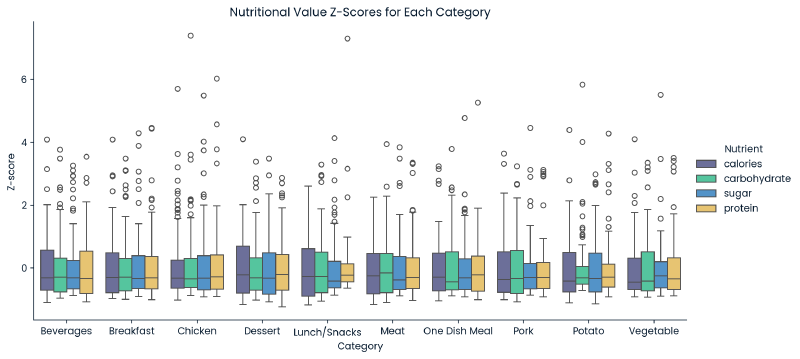
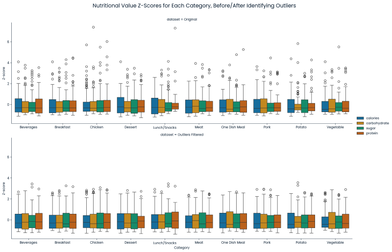
calories,carbohydrate,sugar, andprotein) had 52 rows in common that had missing nutritional values. Since this data was not Missing Completely at Random, the values could not be imputed without introducing bias. As a result, these 52 records were removed. - Each nutritional value initially appeared to have outliers. These outliers were identified by iterating through each nutritient’s ‘category’ values to find outliers outside of the 1.5x the interquartile range (IQR) for each category. It was found that these compromised of ~19% of the dataset. Due to the large proportion of the data, and because they did not seem to be input errors, they were left as is (no change).
- The distribution of these nutritional values will be explored further during Exploratory Analysis.
1 cell collapsed:
## updated this so bottom graph uses filtered_df instead of cleaned_df, since outliers are not being removed.

# apply z-scores, per category
original_grouped_z_scores = df.groupby('category')[['calories', 'carbohydrate', 'sugar', 'protein']].transform(calculate_z_scores_by_category)
cleaned_grouped_z_scores = filtered_df.groupby('category')[['calories', 'carbohydrate', 'sugar', 'protein']].transform(calculate_z_scores_by_category)

# add 'category' column
original_grouped_z_scores['category'] = df['category']
cleaned_grouped_z_scores['category'] = filtered_df['category']

# melt the dataframes for plotting
original_melted = original_grouped_z_scores.melt(id_vars=['category'], value_vars=['calories', 'carbohydrate', 'sugar', 'protein'],
                                                 var_name='Nutrient', value_name='Z-score')
cleaned_melted = cleaned_grouped_z_scores.melt(id_vars=['category'], value_vars=['calories', 'carbohydrate', 'sugar', 'protein'],
                                               var_name='Nutrient', value_name='Z-score')
# concat data
data = pd.concat([original_melted.assign(dataset='Original'), cleaned_melted.assign(dataset='Outliers Filtered')], ignore_index=True)

# map boxplots to data
g = sns.FacetGrid(data, row="dataset", height=5, aspect=3, sharex=False)
g.map_dataframe(sns.boxplot, x='category', y='Z-score', hue='Nutrient', palette='colorblind')
g.set_xticklabels(rotation=0)
g.set_axis_labels("Category", "Z-score")
g.add_legend()

g.fig.suptitle('Nutritional Value Z-Scores for Each Category, Before/After Identifying Outliers', fontsize=16, y=1.05)

plt.show()
Post Data Cleaning #
- 895 entries remained after data cleaning.
- An analysis was done of the target variable’s distribution via a two-sample Kolmogorov-Smirnov test. This analysis determined that there was not a statistical difference in the target variable’s distribution due to the data cleaning.
Input collapsed:
# determine if target variable distribution differs signficantly due to removed outliers
ks_stat, ks_p = ks_2samp(df['high_traffic'], cleaned_df['high_traffic'])
if ks_p < 0.05:
    sig = 'The distributions are signficantly different'
else:
    sig = 'No statistical difference in the distributions. '
print(f'KS Statistic (high_traffic): {ks_stat}, P-value: {ks_p}. {sig}')
KS Statistic (high_traffic): 0.008359240884179974, P-value: 0.9999999999999847. No statistical difference in the distributions.
2. Exploratory Analysis #
I have investigated the target variable and features of the recipes, as well as the relationship between the target variable and features. After the analysis the following changes were identified to enable modeling:
- Protein: use log transformation due to statistical significance as a predictor for
high_traffic
Target Variable - High Traffic #
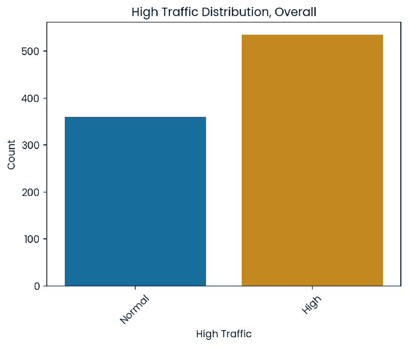
Our goal is to be able to predict instances of high traffic on the website meaning our target variable is high_traffic. When looking at the overall counts of high traffic there are over 500 instances of high traffic with approximately 350 showing normal traffic.
Input collapsed:
# overal count plot
sns.countplot(x='high_traffic', hue='high_traffic', data=cleaned_df, palette='colorblind', dodge=False)
plt.title('High Traffic Distribution, Overall')
plt.xticks(ticks=[0,1],labels=['Normal', 'High'], rotation=45)
plt.xlabel('High Traffic')
plt.ylabel('Count')
plt.legend().remove()
plt.show()
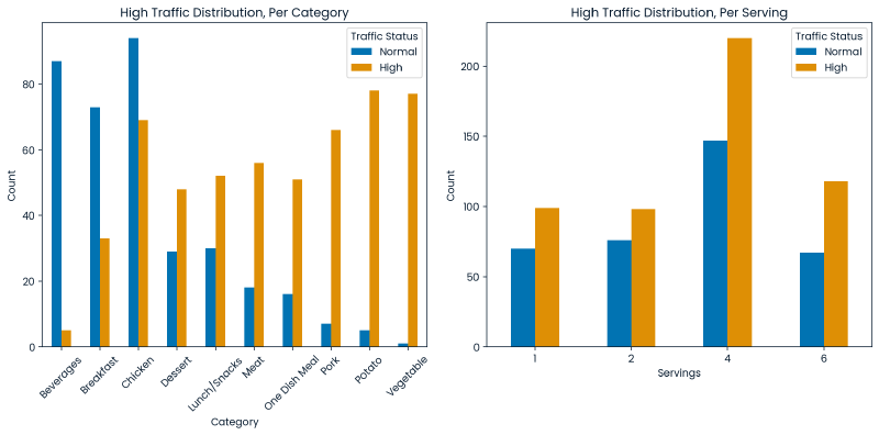
Below are two graphs:
- (Left) When the target variable is broken out by category we can also observe that some categories more frequently produce a state of high traffic which suggests a relationship between the the recipe’s category and our target variable.
- (Right) When the target variable is counted on a basis of serving size, it does not appear that the serving size has a strong relationship with the target variable.
Input collapsed:
plt.figure(figsize=(12, 6))

# prepare data
category_counts = pd.crosstab(cleaned_df['category'], cleaned_df['high_traffic'])

# high traffic vs category
ax1 = plt.subplot(1, 2, 1)
category_counts.plot(kind='bar', color=sns.color_palette("colorblind"), stacked=False, ax=ax1)
plt.title('High Traffic Distribution, Per Category')
plt.xlabel('Category')
plt.ylabel('Count')
plt.xticks(rotation=45)
plt.legend(title='Traffic Status', labels=['Normal', 'High'])

category_counts = pd.crosstab(cleaned_df['servings'], cleaned_df['high_traffic'])

# high traffic vs servings
ax2 = plt.subplot(1, 2, 2)
category_counts.plot(kind='bar', color=sns.color_palette("colorblind"), stacked=False, ax=ax2)
plt.title('High Traffic Distribution, Per Serving')
plt.xlabel('Servings')
plt.ylabel('Count')
plt.xticks(rotation=0)
plt.legend(title='Traffic Status', labels=['Normal', 'High'])


plt.tight_layout()
plt.show()
Numeric Variables - Calories, Carbohydrate, Sugar, Protein #
The below are histplots and boxplots for the numeric variables to get a sense of their distributions.
Input collapsed:
plt.figure(figsize=(12, 18))

ax1 = plt.subplot(4, 2, 1)
sns.histplot(data=cleaned_df, x='calories', kde=True, ax=ax1)
plt.title('Calories, Histplot')

ax2 = plt.subplot(4, 2, 2)
sns.boxplot(data=cleaned_df, y='calories', ax=ax2)
plt.title('Calories, Boxplot')

ax3 = plt.subplot(4, 2, 3)
sns.histplot(data=cleaned_df, x='carbohydrate', kde=True, ax=ax3)
plt.title('Carbohydrate, Histplot')

ax4 = plt.subplot(4, 2, 4)
sns.boxplot(data=cleaned_df, y='carbohydrate', ax=ax4)
plt.title('Carbohydrate, Boxplot')

ax5 = plt.subplot(4, 2, 5)
sns.histplot(data=cleaned_df, x='sugar', kde=True, ax=ax5)
plt.title('Sugar, Histplot')

ax6 = plt.subplot(4, 2, 6)
sns.boxplot(data=cleaned_df, y='sugar', ax=ax6)
plt.title('Sugar, Boxplot')

ax7 = plt.subplot(4, 2, 7)
sns.histplot(data=cleaned_df, x='protein', kde=True, ax=ax7)
plt.title('Protein, Histplot')

ax8 = plt.subplot(4, 2, 8)
sns.boxplot(data=cleaned_df, y='protein', ax=ax8)
plt.title('Protein, Boxplot')

plt.tight_layout()
plt.show()
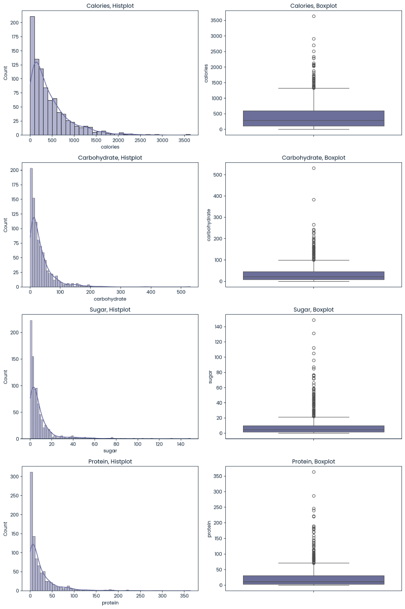
Conclusions -
- Due to the right-skewed nature of distributions, a log transformation of these variables will be investigated as well.
- While there are values that exist outside of the IQR for these nutritional values, they do generally appear alongside a range of acceptable values. Some values appear to be extreme but not to the point of being misentered. No outliers will be removed.
Relationship between Numerical Values and High Traffic #
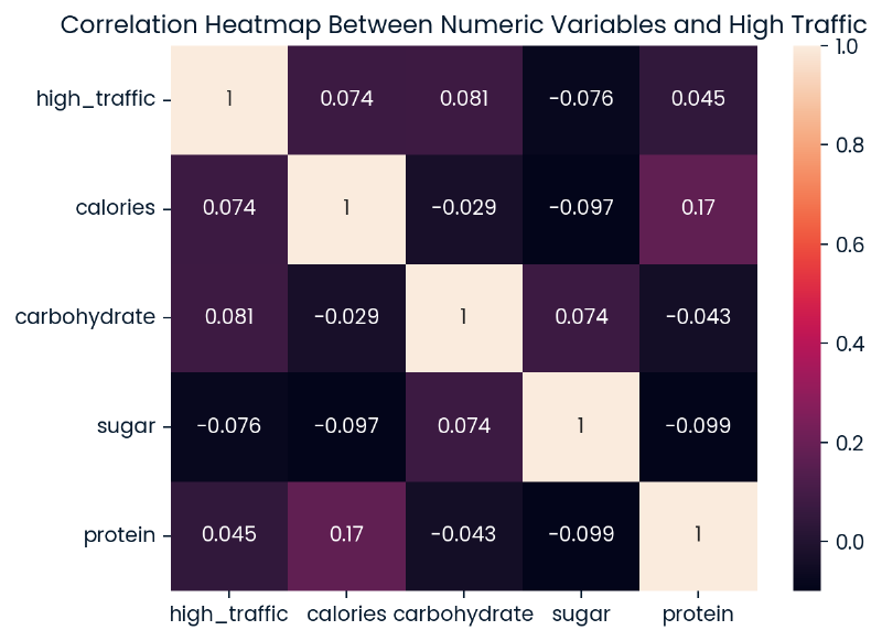
Below is a heatmap of the relationships between the nutritional values and high_traffic. The strongest relationship displayed is between calories and protein showing a positive low correlation. Looking at the relationships with high_traffic specifically, it does appear that there are several other low correlations when nutritional values are used as predictors for the target variable.
Input collapsed:
# numeric heatmap
heatmap_vals = ['high_traffic'] + nutrient_vals
numeric_vals = nutrient_vals
numeric = cleaned_df[heatmap_vals]
sns.heatmap(numeric.corr(),annot=True).set(title='Correlation Heatmap Between Numeric Variables and High Traffic')
plt.show()
2 cells collapsed:
# compile correlation data into dataframe
correlation_data = []

# linear correlations with 'high_traffic'
for col in numeric_vals:
    correlation, p_value = pointbiserialr(cleaned_df['high_traffic'], cleaned_df[col])
    correlation_data.append({'Variable': col, 'Type': 'Original', 'Correlation': correlation, 'P-Value': p_value})
    print(f"{col} to high_traffic correlation: {correlation:.4f} (P-value: {p_value:.4f})")

# linear correlations with 'high_traffic', per category
for cat in cleaned_df['category'].unique():
    category_df = cleaned_df[cleaned_df['category'] == cat]
    for col in numeric_vals:
        correlation, p_value = pointbiserialr(category_df['high_traffic'], category_df[col])
        print(f"{cat},{col} to high_traffic correlation: {correlation:.4f} (P-value: {p_value:.4f})")
calories to high_traffic correlation: 0.0744 (P-value: 0.0261)
carbohydrate to high_traffic correlation: 0.0809 (P-value: 0.0154)
sugar to high_traffic correlation: -0.0755 (P-value: 0.0238)
protein to high_traffic correlation: 0.0446 (P-value: 0.1828)
Potato,calories to high_traffic correlation: -0.1760 (P-value: 0.1114)
Potato,carbohydrate to high_traffic correlation: 0.0353 (P-value: 0.7514)
Potato,sugar to high_traffic correlation: -0.0946 (P-value: 0.3951)
Potato,protein to high_traffic correlation: 0.1201 (P-value: 0.2796)
Breakfast,calories to high_traffic correlation: -0.0263 (P-value: 0.7888)
Breakfast,carbohydrate to high_traffic correlation: -0.0991 (P-value: 0.3121)
Breakfast,sugar to high_traffic correlation: 0.0169 (P-value: 0.8635)
Breakfast,protein to high_traffic correlation: -0.0495 (P-value: 0.6142)
Beverages,calories to high_traffic correlation: -0.0679 (P-value: 0.5203)
Beverages,carbohydrate to high_traffic correlation: 0.0177 (P-value: 0.8670)
Beverages,sugar to high_traffic correlation: 0.0036 (P-value: 0.9732)
Beverages,protein to high_traffic correlation: -0.1356 (P-value: 0.1976)
One Dish Meal,calories to high_traffic correlation: 0.1038 (P-value: 0.4031)
One Dish Meal,carbohydrate to high_traffic correlation: 0.1627 (P-value: 0.1885)
One Dish Meal,sugar to high_traffic correlation: 0.0017 (P-value: 0.9888)
One Dish Meal,protein to high_traffic correlation: 0.0691 (P-value: 0.5787)
Chicken,calories to high_traffic correlation: 0.0100 (P-value: 0.8993)
Chicken,carbohydrate to high_traffic correlation: -0.0175 (P-value: 0.8246)
Chicken,sugar to high_traffic correlation: -0.0598 (P-value: 0.4480)
Chicken,protein to high_traffic correlation: 0.0981 (P-value: 0.2130)
Lunch/Snacks,calories to high_traffic correlation: 0.0520 (P-value: 0.6425)
Lunch/Snacks,carbohydrate to high_traffic correlation: -0.0492 (P-value: 0.6604)
Lunch/Snacks,sugar to high_traffic correlation: -0.1447 (P-value: 0.1947)
Lunch/Snacks,protein to high_traffic correlation: -0.1902 (P-value: 0.0870)
Pork,calories to high_traffic correlation: 0.0216 (P-value: 0.8560)
Pork,carbohydrate to high_traffic correlation: 0.0530 (P-value: 0.6563)
Pork,sugar to high_traffic correlation: 0.0564 (P-value: 0.6358)
Pork,protein to high_traffic correlation: 0.0207 (P-value: 0.8619)
Vegetable,calories to high_traffic correlation: 0.0788 (P-value: 0.4927)
Vegetable,carbohydrate to high_traffic correlation: 0.0802 (P-value: 0.4854)
Vegetable,sugar to high_traffic correlation: 0.0896 (P-value: 0.4355)
Vegetable,protein to high_traffic correlation: -0.0975 (P-value: 0.3956)
Meat,calories to high_traffic correlation: -0.1497 (P-value: 0.2031)
Meat,carbohydrate to high_traffic correlation: 0.1484 (P-value: 0.2070)
Meat,sugar to high_traffic correlation: 0.1269 (P-value: 0.2813)
Meat,protein to high_traffic correlation: -0.0195 (P-value: 0.8692)
Dessert,calories to high_traffic correlation: 0.1325 (P-value: 0.2506)
Dessert,carbohydrate to high_traffic correlation: 0.0434 (P-value: 0.7079)
Dessert,sugar to high_traffic correlation: -0.0970 (P-value: 0.4012)
Dessert,protein to high_traffic correlation: -0.0618 (P-value: 0.5936)
# apply log transformation
cleaned_df_log = cleaned_df.copy()
for col in numeric_vals:
    cleaned_df_log[col] = np.log(cleaned_df_log[col] + 1)

# log correlation with  'high_traffic'
for col in numeric_vals:
    correlation, p_value = pointbiserialr(cleaned_df_log['high_traffic'], cleaned_df_log[col])
    correlation_data.append({'Variable': col, 'Type': 'Log-Transformed', 'Correlation': correlation, 'P-Value': p_value})
    print(f"Log-transformed {col} to high_traffic correlation: {correlation:.4f} (P-value: {p_value:.4f})")
# log correlation with 'high_traffic', per category
for cat in cleaned_df_log['category'].unique():
    category_df = cleaned_df_log[cleaned_df_log['category'] == cat]
    for col in numeric_vals:
        correlation, p_value = pointbiserialr(category_df['high_traffic'], category_df[col])
        print(f"{cat}, Log-transformed {col} to high_traffic correlation: {correlation:.4f} (P-value: {p_value:.4f})")
Log-transformed calories to high_traffic correlation: 0.0620 (P-value: 0.0636)
Log-transformed carbohydrate to high_traffic correlation: 0.0602 (P-value: 0.0720)
Log-transformed sugar to high_traffic correlation: -0.0735 (P-value: 0.0278)
Log-transformed protein to high_traffic correlation: 0.1337 (P-value: 0.0001)
Potato, Log-transformed calories to high_traffic correlation: -0.1889 (P-value: 0.0873)
Potato, Log-transformed carbohydrate to high_traffic correlation: -0.0192 (P-value: 0.8630)
Potato, Log-transformed sugar to high_traffic correlation: -0.0558 (P-value: 0.6164)
Potato, Log-transformed protein to high_traffic correlation: 0.1382 (P-value: 0.2127)
Breakfast, Log-transformed calories to high_traffic correlation: -0.0300 (P-value: 0.7598)
Breakfast, Log-transformed carbohydrate to high_traffic correlation: -0.1388 (P-value: 0.1560)
Breakfast, Log-transformed sugar to high_traffic correlation: 0.0065 (P-value: 0.9472)
Breakfast, Log-transformed protein to high_traffic correlation: 0.0035 (P-value: 0.9718)
Beverages, Log-transformed calories to high_traffic correlation: -0.1281 (P-value: 0.2238)
Beverages, Log-transformed carbohydrate to high_traffic correlation: 0.0390 (P-value: 0.7121)
Beverages, Log-transformed sugar to high_traffic correlation: 0.0279 (P-value: 0.7920)
Beverages, Log-transformed protein to high_traffic correlation: -0.1397 (P-value: 0.1841)
One Dish Meal, Log-transformed calories to high_traffic correlation: 0.0144 (P-value: 0.9079)
One Dish Meal, Log-transformed carbohydrate to high_traffic correlation: 0.0352 (P-value: 0.7770)
One Dish Meal, Log-transformed sugar to high_traffic correlation: -0.0075 (P-value: 0.9522)
One Dish Meal, Log-transformed protein to high_traffic correlation: 0.0606 (P-value: 0.6260)
Chicken, Log-transformed calories to high_traffic correlation: 0.0912 (P-value: 0.2467)
Chicken, Log-transformed carbohydrate to high_traffic correlation: -0.0441 (P-value: 0.5759)
Chicken, Log-transformed sugar to high_traffic correlation: -0.0461 (P-value: 0.5587)
Chicken, Log-transformed protein to high_traffic correlation: 0.0905 (P-value: 0.2505)
Lunch/Snacks, Log-transformed calories to high_traffic correlation: -0.0654 (P-value: 0.5591)
Lunch/Snacks, Log-transformed carbohydrate to high_traffic correlation: -0.0488 (P-value: 0.6635)
Lunch/Snacks, Log-transformed sugar to high_traffic correlation: -0.1156 (P-value: 0.3009)
Lunch/Snacks, Log-transformed protein to high_traffic correlation: -0.1991 (P-value: 0.0730)
Pork, Log-transformed calories to high_traffic correlation: -0.0425 (P-value: 0.7211)
Pork, Log-transformed carbohydrate to high_traffic correlation: -0.0765 (P-value: 0.5201)
Pork, Log-transformed sugar to high_traffic correlation: 0.0076 (P-value: 0.9491)
Pork, Log-transformed protein to high_traffic correlation: -0.0119 (P-value: 0.9206)
Vegetable, Log-transformed calories to high_traffic correlation: 0.0669 (P-value: 0.5604)
Vegetable, Log-transformed carbohydrate to high_traffic correlation: 0.0782 (P-value: 0.4963)
Vegetable, Log-transformed sugar to high_traffic correlation: 0.1443 (P-value: 0.2074)
Vegetable, Log-transformed protein to high_traffic correlation: -0.1274 (P-value: 0.2664)
Meat, Log-transformed calories to high_traffic correlation: -0.1949 (P-value: 0.0961)
Meat, Log-transformed carbohydrate to high_traffic correlation: 0.1384 (P-value: 0.2395)
Meat, Log-transformed sugar to high_traffic correlation: 0.1779 (P-value: 0.1294)
Meat, Log-transformed protein to high_traffic correlation: 0.0125 (P-value: 0.9156)
Dessert, Log-transformed calories to high_traffic correlation: 0.1106 (P-value: 0.3383)
Dessert, Log-transformed carbohydrate to high_traffic correlation: 0.0535 (P-value: 0.6439)
Dessert, Log-transformed sugar to high_traffic correlation: 0.0244 (P-value: 0.8332)
Dessert, Log-transformed protein to high_traffic correlation: 0.0312 (P-value: 0.7874)
Since the distributions of the numeric variables were skewed, a logarithmic transformation was applied to these variables to explore if this improved relationships with the target variable.
Below are two heatmaps:
- Correlations (left)
- P-Values (right).
Each heatmap further explores the log-transformed nutrional values and original values in relationship with high_traffic.
Input collapsed:
## heatmaps for correlation and p-values
# convert correlation data to dataframe
correlation_df = pd.DataFrame(correlation_data)

# plot
fig, ax = plt.subplots(1, 2, figsize=(16, 6))

# correlation
correlation_pivot = correlation_df.pivot("Variable", "Type", "Correlation")
sns.heatmap(correlation_pivot, annot=True, fmt=".3f", cmap='vlag', center=0, vmin=-1, vmax=1, ax=ax[0])
ax[0].set_title('Correlation of Numeric Values with High Traffic')

# p-value
correlation_pivot = correlation_df.pivot("Variable", "Type", "P-Value")
sns.heatmap(correlation_pivot, annot=True, fmt=".4f", cmap='vlag_r', center=0.5, vmin=0, vmax=1, ax=ax[1])
ax[1].set_title('P-Values of Numeric Values with High Traffic')

plt.show()
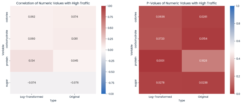
Conclusions -
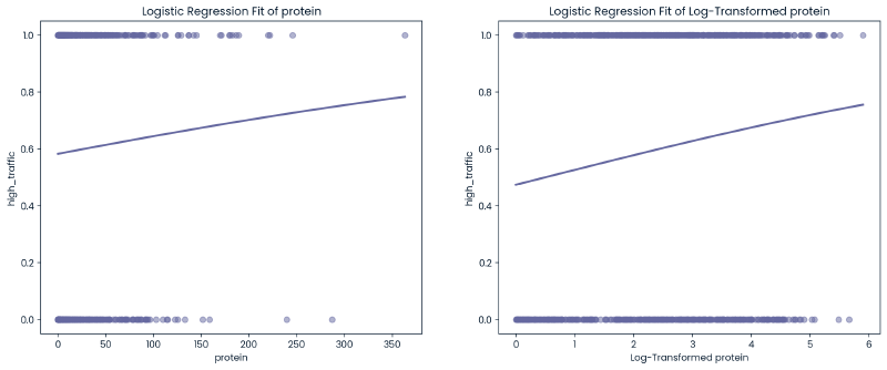
- The log-transformed protein displayed an improvement in correlation with
high_traffic, and this log-transformed protein now is statistically significant in predicting the target variable. - While other log-transformed values have a P-value < 0.05 showing statistical significance, the original values for
calories,carbohydrate, andsugarare more signficant in predictinghigh_trafficthan their log-transformed counterparts.
1 cell collapsed:
def plot_logistic_fit(data, x, y, axn, transformed=False, ):
    sns.regplot(x=x, y=y, data=data, logistic=True, ci=None, scatter_kws={'alpha':0.5}, ax=ax[axn])
    title = 'Logistic Regression Fit of ' + ('Log-Transformed ' if transformed else '') + x
    ax[axn].set_title(title)
    plt.xlabel('Log-Transformed ' + x if transformed else x)
    plt.ylabel(y)

fig, ax = plt.subplots(1, 2, figsize=(16, 6))
plot_logistic_fit(cleaned_df, 'protein', 'high_traffic', axn=0)
plot_logistic_fit(cleaned_df_log, 'protein', 'high_traffic', axn=1,transformed=True)
plt.show()
Categorical Variable - Category, Servings #
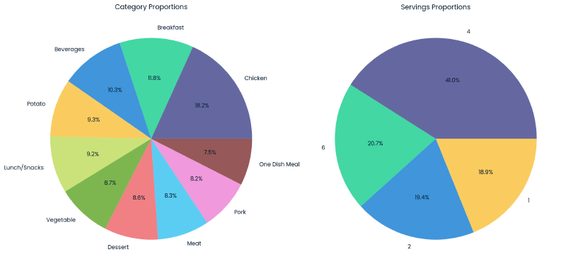
The category variable fairly uniformly distributed with most categories representing between 7.5-10.3% of the dataset. Notable exceptions include ‘Breakfast’ which represents 11.8% of the data, and ‘Chicken’ which represents 18.2% of the data making it the most prevalent category.
For servings, recipes with 4+ servings account for ~61.7%, with the remainder of recipes having a serving size of 1 or 2.
Input collapsed:
fig, ax = plt.subplots(1, 2, figsize=(14, 7))

# pie chart for 'category'
cleaned_df['category'].value_counts().plot.pie(autopct='%1.1f%%', ax=ax[0])
ax[0].set_title('Category Proportions')
ax[0].set_ylabel('')


# pie chart for 'serving'
cleaned_df['servings'].value_counts().plot.pie(autopct='%1.1f%%',ax=ax[1])
ax[1].set_title('Servings Proportions')
ax[1].set_ylabel('')

plt.tight_layout()
plt.show()
Relationship between Category and High Traffic #
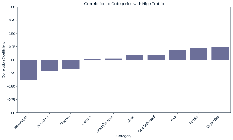
As discussed under the target variable section, some categories more frequently produce a state of high traffic indicating that the category variable may be useful in our modeling as a predictor when combined with numeric variables.
The below are two heatmaps for correlation and p-values, broken out by each category value.
1 cell collapsed:
# dummy categories
category_dummies = pd.get_dummies(cleaned_df['category'])

categories = []
correlations = []
p_values = []

# calc corr and p-value
for column in category_dummies:
    corr, p_val = pointbiserialr(category_dummies[column], cleaned_df['high_traffic'])
    categories.append(column)
    correlations.append(corr)
    p_values.append(p_val)

# store results in idf
results_df_cleaned = pd.DataFrame({
    'Category': categories,
    'Correlation': correlations,
    'P-Value': p_values
})

# correlation bar chart with p-values
fig, ax = plt.subplots(figsize=(12, 6))
bars = sns.barplot(x='Category', y='Correlation', data=results_df_cleaned, ax=ax)
ax.set_title('Correlation of Categories with High Traffic')
ax.set_ylabel('Correlation Coefficient')
ax.set_ylim([-1, 1])
ax.set_xticklabels(results_df_cleaned['Category'], rotation=45, ha="right")

"""
# p-value anotations
for bar, p_value in zip(bars.patches, results_df_cleaned['P-Value']):
    y = bar.get_height()
    x = bar.get_x() + bar.get_width() / 2
    ax.text(x, y, f'p={p_value:.9f}', ha='center', va='bottom' if y >= 0 else 'top', color='black', fontsize=9)
"""
plt.show()
Input collapsed:
# dummy categories
category_dummies = pd.get_dummies(cleaned_df['category'])
cat_corr_df = pd.concat([cleaned_df, category_dummies], axis=1)
categories = []
correlations = []
p_values = []

# calculate correlation and p-values for each category
for column in category_dummies.columns:
    correlation, p_value = pointbiserialr(cat_corr_df[column], cat_corr_df['high_traffic'])
    categories.append(column)
    correlations.append(correlation)
    p_values.append(p_value)

# create dataframe
correlation_df = pd.DataFrame({
    'Category': categories,
    'Correlation': correlations,
    'P-Value': p_values
})

# plot
fig, ax = plt.subplots(1, 2, figsize=(16, 6))

# corr
correlation_matrix = correlation_df.pivot_table(index='Category', values='Correlation', aggfunc='sum')
sns.heatmap(correlation_matrix, annot=True, fmt=".3f", cmap='vlag', ax=ax[0])
ax[0].set_title('Correlation of Categories with High Traffic')

# p-value
p_values_matrix = correlation_df.pivot_table(index='Category', values='P-Value', aggfunc='sum')
sns.heatmap(p_values_matrix, annot=True, cmap='vlag_r', center=0.5, vmin=0, vmax=1, ax=ax[1])
ax[1].set_title('P-Values of Categories with High Traffic')

plt.tight_layout()
plt.show()
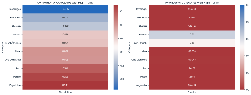
Conclusion - There are many minor correlations between category values and high_traffic. Each category value, except Dessert and Lunch/Snacks, display statistical signficance in predicting our target variable.
Relationship between Servings and High Traffic #
Under the discussion for the target variable it did not appear there was a strong relationship between servings and high_traffic. Below is a correlation and p-value calculation between these two variables.
correlation, p_value = pointbiserialr(cleaned_df['high_traffic'], cleaned_df['servings'])
print(f"Correlation: {correlation:.4f} \nP-value: {p_value:.4f}")
Correlation: 0.0432
P-value: 0.1963
Conclusion - There is only a minor positive correlation between servings and high_traffic but this is not enough to be considered statistically signficant.
3. Model Development #
The goal of predicting high_traffic is a binary classification problem.
For my models I am choosing:
- Logistic Regression: This is a linear model well-suited for binary classification problems. It was chosen due to the presence of statistically significant predictors among our features, which aligns well with the logistic regression approach.
- Random Forest Classifier as a comparison model. This ensemble method, which utilizes multiple decision trees, was selected for its ability to model complex interactions between variables and its robustness to various input data distributions. It is particularly suitable for exploring non-linear relationships that may exist within the dataset, which could be missed by linear models.
1 cell collapsed:
from sklearn.model_selection import train_test_split, GridSearchCV, StratifiedKFold
from sklearn.preprocessing import OneHotEncoder, FunctionTransformer, MinMaxScaler
from sklearn.compose import ColumnTransformer
from sklearn.pipeline import Pipeline
from sklearn.impute import SimpleImputer
from sklearn.ensemble import RandomForestClassifier
from sklearn.linear_model import LogisticRegression
from sklearn.metrics import classification_report, confusion_matrix, accuracy_score, precision_score
Preprocessing #
To perform modeling, I have chosen calories, carbohydrate, sugar, protein, servings, and category as features, and high_traffic as a target variable. The following changes will be made:
high_traffichas already been binary encoded as part of data validation.- Numeric features will be normalized via MinMaxScaler. MinMaxScaler was selected because it yielded higher precision/accuracy compared to StandardScaler.
proteinwill be log transformed, then normalized via MinMaxScaler.categorywill be one-hot encoded to enable usage in modeling.
# random state
RAND_STATE = 63

# scoring method
SCORING_METHOD = 'precision'

def log_transform(x):
    """Function to apply log transformation"""
    return np.log1p(x)

# identify numeric columns
numeric_features = cleaned_df.select_dtypes(include=['int64','float64']).columns.tolist()
numeric_features.remove('high_traffic')

# create log transformer
log_transformer = FunctionTransformer(log_transform)

# create ColumnTransformer, scales numeric columns and one-hot-encodes category
preprocessor = ColumnTransformer(
    transformers=[
        ('num', MinMaxScaler(), numeric_features),
        ('num_log', Pipeline([
            ('imputer', SimpleImputer(strategy='mean')),
            ('log', log_transformer),
            ('scaler', MinMaxScaler())
        ]), ['protein']), # log transforms protein
        ('cat', OneHotEncoder(), ['category'])
    ],
    remainder='passthrough'
)

# fit and transform
df_preprocessed = preprocessor.fit_transform(cleaned_df)

# convert back to df
columns_transformed = preprocessor.named_transformers_['cat'].get_feature_names_out(['category'])
new_columns = numeric_features + ['protein_log'] + list(columns_transformed) + ['high_traffic']
df_preprocessed = pd.DataFrame(df_preprocessed, columns=new_columns)
df_preprocessed.head()
| recipe | calories | carbohydrate | sugar | protein | servings | protein_log | category_Beverages | category_Breakfast | category_Chicken | category_Dessert | category_Lunch/Snacks | category_Meat | category_One Dish Meal | category_Pork | category_Potato | category_Vegetable | high_traffic | |
|---|---|---|---|---|---|---|---|---|---|---|---|---|---|---|---|---|---|---|
| 0 | 0.000000 | 0.009727 | 0.072645 | 0.004370 | 0.002532 | 0.6 | 0.110598 | 0.0 | 0.0 | 0.0 | 0.0 | 0.0 | 0.0 | 0.0 | 0.0 | 1.0 | 0.0 | 1.0 |
| 1 | 0.001058 | 0.251620 | 0.080413 | 0.020707 | 0.007926 | 0.0 | 0.229875 | 0.0 | 1.0 | 0.0 | 0.0 | 0.0 | 0.0 | 0.0 | 0.0 | 0.0 | 0.0 | 0.0 |
| 2 | 0.002116 | 0.026669 | 0.057561 | 0.259648 | 0.000055 | 0.6 | 0.003357 | 1.0 | 0.0 | 0.0 | 0.0 | 0.0 | 0.0 | 0.0 | 0.0 | 0.0 | 0.0 | 1.0 |
| 3 | 0.003175 | 0.007407 | 0.003431 | 0.005311 | 0.001459 | 0.6 | 0.072102 | 1.0 | 0.0 | 0.0 | 0.0 | 0.0 | 0.0 | 0.0 | 0.0 | 0.0 | 0.0 | 0.0 |
| 4 | 0.004233 | 0.190203 | 0.006467 | 0.011026 | 0.148420 | 0.2 | 0.679207 | 0.0 | 0.0 | 0.0 | 0.0 | 0.0 | 0.0 | 1.0 | 0.0 | 0.0 | 0.0 | 1.0 |
# split into target sets
X = df_preprocessed.drop(['recipe','high_traffic', 'protein'], axis=1)
y = df_preprocessed['high_traffic']

# split into training and test data
X_train, X_test, y_train, y_test = train_test_split(X, y, test_size=0.25, random_state=RAND_STATE)

# maintain proportion of classes
cv = StratifiedKFold(n_splits=10)
Model 1: Logistic Regression #
# define hyperparameter grid
grid = {
    'C': [0.05, 0.1, 0.5, 1],
    'penalty': ["l1", "l2", "elasticnet", None],
    'multi_class': ["auto", "ovr", "multinomial"],
    'solver': ['liblinear', 'lbfgs', 'newton-cg']
}

# grid cross validate and fit
logreg = LogisticRegression(random_state=RAND_STATE)
logreg_cv = GridSearchCV(logreg, grid, cv=cv, scoring=SCORING_METHOD, verbose=1)
logreg_cv.fit(X_train, y_train)

# display results
print(f'Best Score: {logreg_cv.best_score_}')
print(f'Best Hyperparameters: {logreg_cv.best_params_}')
print(f'Std deviation of CV scores for the best hyperparameters: {logreg_cv.cv_results_["std_test_score"][logreg_cv.best_index_]}')
Fitting 10 folds for each of 144 candidates, totalling 1440 fits
Best Score: 0.8015619610356453
Best Hyperparameters: {'C': 0.1, 'multi_class': 'multinomial', 'penalty': 'l2', 'solver': 'lbfgs'}
Std deviation of CV scores for the best hyperparameters: 0.03959207830248714
# unpack best_params to create model
logreg2 = LogisticRegression(**logreg_cv.best_params_, random_state=RAND_STATE)
logreg2.fit(X_train, y_train)
LogisticRegression(C=0.1, multi_class='multinomial', random_state=63)In a Jupyter environment, please rerun this cell to show the HTML representation or trust the notebook.
On GitHub, the HTML representation is unable to render, please try loading this page with nbviewer.org.
LogisticRegression(C=0.1, multi_class='multinomial', random_state=63)
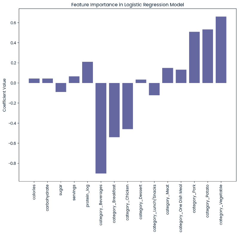
Feature Importance
Input collapsed:
feature_cols = X.columns
resultdict = {}

model = logreg2

if len(model.coef_.shape) > 1:
    coefs = model.coef_[0]
else:
    coefs = model.coef_

for i, col_name in enumerate(feature_cols):
    resultdict[col_name] = coefs[i]

plt.figure(figsize=(10, 8))
plt.bar(resultdict.keys(), resultdict.values())
plt.xticks(rotation=90)
plt.title('Feature Importance in Logistic Regression Model')
plt.ylabel('Coefficient Value')
plt.show()
Model 2: Random Forest Classifier #
# define hyperparameter grid
grid = {
    'n_estimators': range(10, 100, 10),
    'max_depth': range(1, 10)
}

# grid cross validate and fit
rfc = RandomForestClassifier(random_state=RAND_STATE)
rfc_cv = GridSearchCV(rfc, grid, cv=cv, scoring=SCORING_METHOD, verbose=1)
rfc_cv.fit(X_train, y_train)

# display results
print(f'Best Score: {rfc_cv.best_score_}')
print(f'Best Hyperparameters: {rfc_cv.best_params_}')
print(f'Std deviation of CV scores for the best hyperparameters: {rfc_cv.cv_results_["std_test_score"][rfc_cv.best_index_]}')
Fitting 10 folds for each of 81 candidates, totalling 810 fits
Best Score: 0.7750656009793719
Best Hyperparameters: {'max_depth': 8, 'n_estimators': 20}
Std deviation of CV scores for the best hyperparameters: 0.05166332539478016
# unpack best_params to create model
rfc2 = RandomForestClassifier(**rfc_cv.best_params_, random_state=RAND_STATE)
rfc2.fit(X_train, y_train)
RandomForestClassifier(max_depth=8, n_estimators=20, random_state=63)In a Jupyter environment, please rerun this cell to show the HTML representation or trust the notebook.
On GitHub, the HTML representation is unable to render, please try loading this page with nbviewer.org.
RandomForestClassifier(max_depth=8, n_estimators=20, random_state=63)
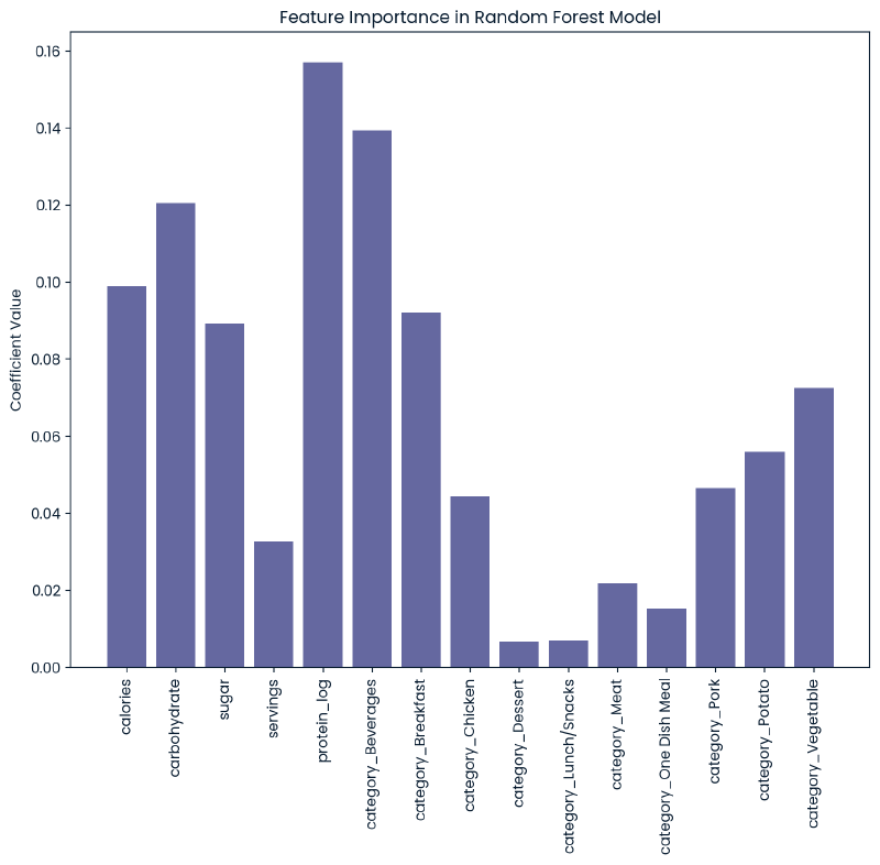
Feature Importance
Input collapsed:
feature_cols = X.columns
resultdict = {}

model = rfc2

importances = model.feature_importances_

for i, col_name in enumerate(feature_cols):
    resultdict[col_name] = importances[i]

plt.figure(figsize=(10, 8))
plt.bar(resultdict.keys(), resultdict.values())
plt.xticks(rotation=90)
plt.title('Feature Importance in Random Forest Model')
plt.ylabel('Coefficient Value')
plt.show()
1 cell collapsed:
# removed to focus on 2 models.
# LinearSVC
"""
# define hyperparameter grid
grid = {
    'C': [0.01, 0.05, 0.1, 0.25, 0.5, 0.75, 1],
    'penalty': ["l1", "l2"],
    'loss': ['hinge','squared_hinge']
}

# grid cross validate and fit
svm = LinearSVC(random_state=RAND_STATE)
svm_cv = GridSearchCV(svm, grid, cv=cv, scoring=SCORING_METHOD, verbose=1)
svm_cv.fit(X_train, y_train)

# display results
print(f'Best Score: {svm_cv.best_score_}')
print(f'Best Hyperparameters: {svm_cv.best_params_}')
print(f'Std deviation of CV scores for the best hyperparameters: {svm_cv.cv_results_["std_test_score"][svm_cv.best_index_]}')

# unpack best_params to create model
svm2 = LinearSVC(**svm_cv.best_params_)
svm2.fit(X_train, y_train)

# evaluate
y_pred_svm = svm2.predict(X_test)

print('Classification report:\n', classification_report(y_test, y_pred_svm))
print('Confusion matrix:\n', confusion_matrix(y_test, y_pred_svm))
"""
'\n# define hyperparameter grid\ngrid = {\n \'C\': [0.01, 0.05, 0.1, 0.25, 0.5, 0.75, 1],\n \'penalty\': ["l1", "l2"],\n \'loss\': [\'hinge\',\'squared_hinge\']\n}\n\n# grid cross validate and fit\nsvm = LinearSVC(random_state=RAND_STATE)\nsvm_cv = GridSearchCV(svm, grid, cv=cv, scoring=SCORING_METHOD, verbose=1)\nsvm_cv.fit(X_train, y_train)\n\n# display results\nprint(f\'Best Score: {svm_cv.best_score_}\')\nprint(f\'Best Hyperparameters: {svm_cv.best_params_}\')\nprint(f\'Std deviation of CV scores for the best hyperparameters: {svm_cv.cv_results_["std_test_score"][svm_cv.best_index_]}\')\n\n# unpack best_params to create model\nsvm2 = LinearSVC(**svm_cv.best_params_)\nsvm2.fit(X_train, y_train)\n\n# evaluate\ny_pred_svm = svm2.predict(X_test)\n\nprint(\'Classification report:\n\', classification_report(y_test, y_pred_svm))\nprint(\'Confusion matrix:\n\', confusion_matrix(y_test, y_pred_svm))\n'
4. Model Evaluation #
For evaluation, precision is used as the primary benchmark for our key performance indicator (KPI), with overall accuracy serving as a secondary benchmark.
- Precision is prioritized because our business objective is to accurately predict instances of high-traffic. Ensuring that predictions of high traffic are reliable (correct in 80% of cases) minimizes the cost of false positives.
- Accuracy provides a measure of the overall effectiveness of the model across both classes of traffic. This metric is chosen for its simplicity and straightforward metric of the overall performance of the model.
Model 1: Logistic Regression #
y_pred_logreg = logreg2.predict(X_test)
results = {
    'Logistic Regression': {
        'Precision': precision_score(y_test, y_pred_logreg),
        'Accuracy': accuracy_score(y_test, y_pred_logreg)
    }
}

print(f"Precision Score: {results['Logistic Regression']['Precision']:.2f}")
print(f"Accuracy Score: {results['Logistic Regression']['Accuracy']:.2f}\n")
print("Classification report:\n", classification_report(y_test, y_pred_logreg))
print("Confusion matrix:\n", confusion_matrix(y_test, y_pred_logreg))
Precision Score: 0.81
Accuracy Score: 0.77

Classification report:
               precision    recall  f1-score   support

         0.0       0.72      0.71      0.72        91
         1.0       0.81      0.81      0.81       133

    accuracy                           0.77       224
   macro avg       0.76      0.76      0.76       224
weighted avg       0.77      0.77      0.77       224

Confusion matrix:
 [[ 65  26]
 [ 25 108]]
Model 2: Random Forest Classifier #
y_pred_rfc = rfc2.predict(X_test)
results['Random Forest'] = {
    'Precision': precision_score(y_test, y_pred_rfc),
    'Accuracy': accuracy_score(y_test, y_pred_rfc)
}

print(f"Precision Score: {results['Random Forest']['Precision']:.2f}")
print(f"Accuracy Score: {results['Random Forest']['Accuracy']:.2f}\n")
print("Classification report:\n", classification_report(y_test, y_pred_rfc))
print("Confusion matrix:\n", confusion_matrix(y_test, y_pred_rfc))
Precision Score: 0.75
Accuracy Score: 0.75

Classification report:
               precision    recall  f1-score   support

         0.0       0.75      0.58      0.65        91
         1.0       0.75      0.86      0.80       133

    accuracy                           0.75       224
   macro avg       0.75      0.72      0.73       224
weighted avg       0.75      0.75      0.74       224

Confusion matrix:
 [[ 53  38]
 [ 18 115]]
Results #
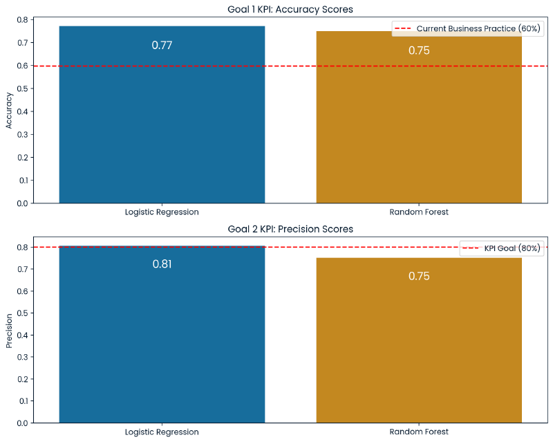
The Logistic Regression model scored 81% precision and 77% accuracy, outperforming the Random Forest Classifier model which scored 75% precision and 75% accuracy. This indicates that the Logistic Regression model is more effective at predicting instances of high traffic with fewer false positives than the Random Forest model. Overall the Logistic Regression model meets the business criteria.
Interestingly, the Random Forest model, despite its slightly lower precision and accuracy, has a higher recall for high traffic predictions (86% compared to Logistic Regression’s 81%). This means that the Random Forest model is able to predict more instances of high traffic but at the cost of more false positives (38 false positives to 26 from the Logistic Regression model). In the business context it is preferable to minimize false positives making precision a more critical KPI than recall. The Random Forest’s tendency to overpredict high traffic could lead to inefficient use of recipes being featured on the website.
Additionally, the Logistic Regression model is linear based and will be able to handle linear relationships among features which fits naturally with the binary classification problem and the linear relationships observed between the recipe’s features. As a result of the linear nature of the model, it will be able to generalize new data better than than the Random Forest model which will help prevent the Logistic Regression model from overfitting.
The Logistic Regression model will provide more balanced performance, meet the business criteria, result in fewer false positives, and is at less risk of overfitting.
5. Business Metrics #
The current business practice of picking recipes to feature on the website results in a state of high traffic approximately 60% of the time.
The business defined two goals:
- Predict which recipes will lead to high traffic?
- Correctly predict high traffic recipes 80% of the time?
The Logistic Regression model meets these requirements. As discussed, its precision score is 81% indicating that when it guesses high traffic it is correct at least 80% of the time. Moreover, the recall and f-1 scores are 81% which means it accurately identifies 81% of all actual high traffic instances. This demonstrates the model’s effectiveness in predicting high traffic scenarios. Additionally, the overall accuracy of the model is 77% meaning that it has a balanced approach when identifying both normal and high traffic.
Going forward, the business should monitor accuracy as a KPI for the first goal, and precision as a KPI for the second goal.
Input collapsed:
models = list(results.keys())
precision_scores = [results[model]['Precision'] for model in models]
accuracy_scores = [results[model]['Accuracy'] for model in models]


fig, axs = plt.subplots(2, 1, figsize=(10, 8), sharex=False)

# accuracy
sns.barplot(x=models, y=accuracy_scores, palette='colorblind', ax=axs[0])
axs[0].axhline(y=0.598, color='r', linestyle='--', label='Current Business Practice (60%)')
axs[0].set_title('Goal 1 KPI: Accuracy Scores')
axs[0].set_ylabel('Accuracy')
axs[0].legend()
for i, score in enumerate(accuracy_scores):
    axs[0].text(i, score - 0.100, f'{score:.2f}', color='white', ha='center', fontsize= 14)

# precision
sns.barplot(x=models, y=precision_scores, palette='colorblind', ax=axs[1])
axs[1].axhline(y=0.8, color='r', linestyle='--', label='KPI Goal (80%)')
axs[1].set_title('Goal 2 KPI: Precision Scores')
axs[1].set_ylabel('Precision')
axs[1].legend()
for i, score in enumerate(precision_scores):
    axs[1].text(i, score - 0.100, f'{score:.2f}', color='white', ha='center', fontsize= 14)

plt.tight_layout()
plt.show()
6. Recommendations #
To predict recipes that produce a state of high traffic across the website, we can deploy the Logistic Regression Model into production. By implementing this model it will be able to predict instances of high traffic correctly 81% of the time. This will benefit the company by more consistently driving web traffic throughout the site.
To implement the model, I recommend the following steps to ensure it is effective and improved regularly:
- Predictive Functionality: Implement predictive functionality for a single recipe, or batch of recipes, that returns the traffic predictions.
- Monitor: Monitor results and update recipe’s
high_trafficstatus with the actual result so accuracy and precision can be improved over time. If KPIs fall below goal then this could trigger a review to investigate. - Validate and Sanitize Input: The database storing the recipe data should validate and sanitize data on input so that the data is consistent across the company. The data validation section of this report found several areas where there was missing data, or data that was unexpected. While data was validated and cleaned for modeling, variations of these errors could repeat in the future without stronger input validation/sanitation.
- Provide More Data: The example recipes had some data that was not provided, such as the recipe’s name, ‘Time to make’ and ‘Cost per serving’. This could be valuable data for the model, as well as potentionally the ingredients. Specifically the time should be split into prep time and cook time as these are important components of prospective recipes. Recipes could also be labeled based on their diet (such as gluten-free, vegetarian, and vegan) which could be important based off of the ‘Vegetable’ category’s importance in predicting high traffic. With additional data the model may be able to learn new connections to enhance its predictions.
- Continuously Improve: Define a regularly occuring interval for the model to be reviewed and improved. Additional data can be ingested and the models performances can be monitored to ensure they meet business KPI’s and are improving over time. I recommend reviewing every few months initially and as the model matures this could be updated to every 6-12 months.
- Document: The model should be documented in terms of its usage, metrics, and its review interval/process. This documentation will serve as a reference for future use and reviews.
Predictive Functionality #
This is example predictive functionality that prompts the user for a recipe ID and will return a prediction. It can be implemented into a function within production to be able to utilize the Logistic Regression model in identifying High Traffic recipes.
try:
    # get recipe ID
    n = int(input('Enter Recipe ID: '))

    # locate and predict
    X_query = X_test.iloc[[n]]
    y_pred_query = logreg2.predict(X_query)

    # print result
    if y_pred_query[0] == 1:
        print('The recipe will produce a state of High Traffic')
    else:
        print('The recipe will result in Normal Traffic')

except ValueError:
    print('Invalid input: Please enter a valid integer for the Recipe ID.')
except IndexError:
    print('Invalid Recipe ID: Please enter a Recipe ID within the valid range.')
Enter Recipe ID: 5
The recipe will produce a state of High Traffic
