
Background #
I volunteered with DataKind during their 2024 datakit focused on affordable housing.
The following is a relatively basic geospatial map for some natural disaster data.
import folium
from folium import FeatureGroup, LayerControl
from folium.plugins import HeatMap, MiniMap
from branca.colormap import LinearColormap
from folium.features import GeoJsonTooltip
import pandas as pd
import geopandas as gpd
# google sheet by David E
document_id = '1EIHK3lGBfIWVhOKcW5QJjjHdhrMeiitwzt3Oh6kugJ4'
tab_name = 'data_1-FL'
url = f'https://docs.google.com/spreadsheets/d/{document_id}/gviz/tq?tqx=out:csv&sheet={tab_name}'

df = pd.read_csv(url)

df.head()
| geoid | Lat | Lon | geoid_year | state | county | state_fips_code | county_fips_code | b19083_001e | b19083_001m | economic_distress_pop_agg | economic_distress_simple_agg | investment_areas | opzone | b23025_002e | b23025_002m | b23025_004e | b23025_004m | b23025_005e | b23025_005m | b23025_006e | b23025_006m | s1701_c03_001e | s1701_c03_001m | s1701_c03_002e | s1701_c03_002m | s1701_c03_003e | s1701_c03_003m | s1701_c03_004e | s1701_c03_004m | s1701_c03_006e | s1701_c03_006m | s1701_c03_007e | s1701_c03_007m | s1701_c03_008e | s1701_c03_008m | s1701_c03_009e | s1701_c03_009m | s1701_c03_010e | s1701_c03_010m | ... | s0101_c02_028m | s0101_c04_028e | s0101_c04_028m | s0101_c06_028e | s0101_c06_028m | s0101_c02_029e | s0101_c02_029m | s0101_c04_029e | s0101_c04_029m | s0101_c06_029e | s0101_c06_029m | s0101_c02_030e | s0101_c02_030m | s0101_c04_030e | s0101_c04_030m | s0101_c06_030e | s0101_c06_030m | s0101_c02_031e | s0101_c02_031m | s0101_c04_031e | s0101_c04_031m | s0101_c06_031e | s0101_c06_031m | loan_amount | median_mortgage_amount | median_prop_value | median_sba504_loan_amount | median_sba7a_loan_amount | num_mortgage | num_mortgage_denials | num_mortgage_originated | number_of_sba504_loans | number_of_sba7a_loans | qct | s2503_c01_024e | s2503_c01_024m | s2503_c03_024e | s2503_c03_024m | s2503_c05_024e | s2503_c05_024m | |
|---|---|---|---|---|---|---|---|---|---|---|---|---|---|---|---|---|---|---|---|---|---|---|---|---|---|---|---|---|---|---|---|---|---|---|---|---|---|---|---|---|---|---|---|---|---|---|---|---|---|---|---|---|---|---|---|---|---|---|---|---|---|---|---|---|---|---|---|---|---|---|---|---|---|---|---|---|---|---|---|---|---|
| 0 | 12001000202 | 29.646160 | -82.332953 | 2020 | 12 | 1 | 12 | 1 | 0.5956 | 0.0799 | YES | YES | YES | 1 | 1890 | 453 | 1837 | 458 | 53 | 43 | 0 | 21 | 75.3 | 9.9 | 100.0 | 95.0 | -666666666.0 | -222222222.0 | 100.0 | 95.0 | 75.6 | 9.9 | 76.5 | 9.9 | 58.8 | 28.2 | 54.0 | 42.5 | 61.7 | 51.3 | ... | 1.7 | 2.7 | 2.6 | 3.6 | 2.4 | 2.7 | 1.6 | 1.9 | 2.2 | 3.2 | 2.4 | 2.1 | 1.6 | 1.2 | 1.9 | 2.6 | 2.4 | 0.0 | 0.9 | 0.0 | 2.6 | 0.0 | 1.4 | 6543.333333 | 205000.0 | 325000.0 | NaN | 150000.0 | 36.0 | 4.0 | 23.0 | NaN | 5.0 | 0 | 1100 | 123 | 563 | 542 | 1136 | 171 |
| 1 | 12001000301 | 29.668004 | -82.331418 | 2020 | 12 | 1 | 12 | 1 | 0.4089 | 0.0654 | YES | YES | YES | 0 | 2263 | 458 | 2124 | 455 | 139 | 103 | 0 | 15 | 22.7 | 9.7 | 13.9 | 21.1 | 40.6 | 51.6 | 11.8 | 18.8 | 25.8 | 9.3 | 33.3 | 13.5 | 13.4 | 9.5 | 24.0 | 14.9 | 20.3 | 17.2 | ... | 5.6 | 13.8 | 6.1 | 15.9 | 8.0 | 14.0 | 5.4 | 13.0 | 5.9 | 15.1 | 7.7 | 10.1 | 3.9 | 9.8 | 5.0 | 10.5 | 5.6 | 2.4 | 1.8 | 1.1 | 1.6 | 4.0 | 3.4 | 44290.000000 | 165000.0 | 225000.0 | 351500.0 | 915000.0 | 83.0 | 15.0 | 40.0 | 4.0 | 2.0 | 0 | 852 | 68 | 815 | 141 | 865 | 86 |
| 2 | 12001000400 | 29.679476 | -82.308121 | 2020 | 12 | 1 | 12 | 1 | 0.3928 | 0.0724 | YES | YES | YES | 1 | 2958 | 768 | 2698 | 708 | 260 | 209 | 0 | 21 | 20.4 | 9.8 | 41.0 | 18.9 | 68.9 | 41.6 | 36.8 | 18.5 | 10.9 | 8.7 | 11.8 | 13.3 | 9.8 | 9.0 | 20.8 | 11.2 | 27.2 | 13.6 | ... | 5.1 | 20.2 | 8.6 | 16.1 | 5.4 | 14.4 | 4.4 | 14.1 | 6.8 | 14.7 | 4.8 | 12.6 | 3.7 | 11.2 | 5.1 | 13.8 | 4.6 | 4.4 | 2.3 | 5.0 | 3.5 | 3.9 | 3.2 | 6940.000000 | 135000.0 | 205000.0 | 121000.0 | 1471000.0 | 284.0 | 60.0 | 117.0 | 5.0 | 5.0 | 0 | 961 | 110 | 909 | 67 | 1297 | 405 |
| 3 | 12001000700 | 29.628043 | -82.295782 | 2020 | 12 | 1 | 12 | 1 | 0.5204 | 0.0995 | YES | YES | YES | 1 | 3098 | 622 | 2857 | 600 | 241 | 202 | 0 | 21 | 29.9 | 13.6 | 36.0 | 25.3 | 48.9 | 47.0 | 31.7 | 22.2 | 31.5 | 13.2 | 48.2 | 25.2 | 25.5 | 11.0 | 20.5 | 10.2 | 17.1 | 11.1 | ... | 5.8 | 23.3 | 6.4 | 25.7 | 7.0 | 21.7 | 6.0 | 19.5 | 6.3 | 23.6 | 7.2 | 19.3 | 5.6 | 17.1 | 6.0 | 21.2 | 6.7 | 5.5 | 2.5 | 4.5 | 2.9 | 6.3 | 3.1 | 74871.000000 | 135000.0 | 185000.0 | 140000.0 | NaN | 293.0 | 62.0 | 104.0 | 1.0 | NaN | 0 | 869 | 110 | 818 | 79 | 979 | 255 |
| 4 | 12001000806 | 29.639118 | -82.332207 | 2020 | 12 | 1 | 12 | 1 | 0.5466 | 0.0649 | YES | YES | YES | 0 | 1431 | 326 | 1337 | 313 | 94 | 95 | 0 | 15 | 51.0 | 13.5 | 36.6 | 28.2 | 16.4 | 30.0 | 53.4 | 37.8 | 56.0 | 13.8 | 60.2 | 13.6 | 36.6 | 24.4 | 2.6 | 4.8 | 0.0 | 27.1 | ... | 4.5 | 9.9 | 7.7 | 11.6 | 7.1 | 8.9 | 3.9 | 6.5 | 6.1 | 11.4 | 6.9 | 8.6 | 3.8 | 6.2 | 6.1 | 11.0 | 6.8 | 4.6 | 1.4 | 2.1 | 3.4 | 7.1 | 5.3 | 7990.000000 | 125000.0 | 265000.0 | 250000.0 | NaN | 18.0 | 3.0 | 6.0 | 1.0 | NaN | 1 | 960 | 38 | -666666666 | -222222222 | 971 | 43 |
5 rows × 389 columns
# geojson from arcgis https://www.arcgis.com/home/item.html?id=3c164274a80748dda926a046525da610
# url = 'https://services.arcgis.com/P3ePLMYs2RVChkJx/arcgis/rest/services/USA_Counties_Generalized_Boundaries/FeatureServer/0/query?outFields=*&where=1%3D1&f=geojson' # exceededTransferLimit	true, refining query
url = 'https://services.arcgis.com/P3ePLMYs2RVChkJx/arcgis/rest/services/USA_Counties_Generalized_Boundaries/FeatureServer/0/query?outFields=*&where=STATE_ABBR%3D%27FL%27&f=geojson'

# Read the GeoJSON data into a GeoDataFrame
counties = gpd.read_file(url)

# Print or inspect the counties data
counties.head()
| OBJECTID | NAME | STATE_NAME | STATE_FIPS | FIPS | SQMI | POPULATION | POP_SQMI | STATE_ABBR | COUNTY_FIPS | Shape__Area | Shape__Length | geometry | |
|---|---|---|---|---|---|---|---|---|---|---|---|---|---|
| 0 | 318 | Alachua County | Florida | 12 | 12001 | 968.81 | 278468 | 287.4 | FL | 001 | 0.235556 | 2.085381 | POLYGON ((-82.40526 29.48510, -82.55477 29.481... |
| 1 | 319 | Baker County | Florida | 12 | 12003 | 588.97 | 28259 | 48.0 | FL | 003 | 0.144074 | 1.683327 | POLYGON ((-82.04629 30.13971, -82.14505 30.140... |
| 2 | 320 | Bay County | Florida | 12 | 12005 | 765.78 | 175216 | 228.8 | FL | 005 | 0.179150 | 3.572319 | MULTIPOLYGON (((-85.38475 30.57410, -85.38210 ... |
| 3 | 321 | Bradford County | Florida | 12 | 12007 | 300.49 | 28303 | 94.2 | FL | 007 | 0.070244 | 1.364875 | POLYGON ((-82.04629 30.13971, -82.04367 29.723... |
| 4 | 322 | Brevard County | Florida | 12 | 12009 | 1051.77 | 606612 | 576.8 | FL | 009 | 0.242008 | 5.141660 | MULTIPOLYGON (((-80.78566 28.78519, -80.76242 ... |
# Define the features you want to visualize and their corresponding column names
feature_list = [

    {
        'name': 'Energy Burden',
        'column': 'energy_burden_percentile',
        'enabled': False
    },
    {
        'name': 'Expected Agricultural Loss due to Natural Hazards Heatmap',
        'column': 'expected_agricultural_loss_rate_natural_hazards_risk_index_percentile',
        'enabled': False
    },
    {
        'name': 'Expected Building Loss due to Natural Hazards Heatmap',
        'column': 'expected_building_loss_rate_natural_hazards_risk_index_percentile',
        'enabled': False
    },
    {
        'name': 'Expected Population Loss due to Natural Hazards Heatmap',
        'column': 'expected_population_loss_rate_natural_hazards_risk_index_percentile',
        'enabled': False
    },
    {
        'name': 'Risk of Fire in 30 years Heatmap',
        'column': 'share_of_properties_at_risk_of_fire_in_30_years_percentile',
        'enabled': False
    },
    {
        'name': 'Risk of Flood in 30 years Heatmap',
        'column': 'share_of_properties_at_risk_of_flood_in_30_years_percentile',
        'enabled': False
    }
]

# Prepare required columns
required_columns = {'Lat', 'Lon', 'geoid'} | {f['column'] for f in feature_list}
required_columns = [col['column'] if isinstance(col, dict) else col for col in required_columns]

# clean and reduce data
df_clean = df.dropna(subset=required_columns)
df_clean_reduced = df_clean[required_columns]
# df_clean_reduced.head()
# Create base map
m = folium.Map(location=[df_clean_reduced['Lat'].mean(), df_clean_reduced['Lon'].mean()], zoom_start=7)

# Create shared color scale for percentile data
shared_color_scale = LinearColormap(
    colors=['green', 'yellow', 'red'],
    vmin=0,
    vmax=100,
    caption="Percentile"
)

# Function to create grid
def create_grid(df, feature_column, grid_size=0.1):
    df['lat_bin'] = np.floor(df['Lat'] / grid_size) * grid_size
    df['lon_bin'] = np.floor(df['Lon'] / grid_size) * grid_size
    grid = df.groupby(['lat_bin', 'lon_bin']).agg({
        feature_column: 'mean',
        'geoid': lambda x: x.iloc[0]  # Take the first geoid in the group
    }).reset_index()
    return grid

# Function to get county name from geoid
def get_county_name(geoid):
    county = counties[counties['FIPS'] == str(geoid)[:5]]
    return county['NAME'].iloc[0] if not county.empty else "Unknown County"

# Iterate over features
for feature in feature_list:
    # Create grid
    grid = create_grid(df_clean_reduced, feature['column'])

    # Create feature group
    feature_group = folium.FeatureGroup(name=feature['name'], show=feature['enabled'])

    # Add grid cells to feature group
    for _, row in grid.iterrows():
        value = row[feature['column']]
        county_name = get_county_name(row['geoid'])

        popup_text = f"""
        <b>{feature['name']}</b><br>
        County: {county_name}<br>
        Percentile: {value:.2f}<br>
        Geoid: {row['geoid']}
        """

        folium.CircleMarker(
            location=[row['lat_bin'], row['lon_bin']],
            radius=10,
            popup=folium.Popup(popup_text, max_width=300),
            tooltip=f"{feature['name']} Percentile: {value:.2f}",
            color=shared_color_scale(value),
            fill=True,
            fillColor=shared_color_scale(value),
            fillOpacity=0.7,
            weight=0
        ).add_to(feature_group)

    feature_group.add_to(m)

# Add county boundaries
folium.GeoJson(
    counties,
    name='County Boundaries',
    style_function=lambda feature: {
        'fillColor': 'transparent',
        'color': 'black',
        'weight': 1,
        'fillOpacity': 0.7,
    },
    tooltip=folium.GeoJsonTooltip(
        fields=['NAME'],
        aliases=['County:'],
        localize=True
    )
).add_to(m)

# Add shared color scale legend to map
shared_color_scale.add_to(m)

# Add layer control
folium.LayerControl().add_to(m)

# Add custom JavaScript to toggle legend visibility
legend_toggle_js = """
<script>
document.addEventListener('DOMContentLoaded', function() {
    var legendElement = document.querySelector('.leaflet-bottom.leaflet-right');
    var layerControl = document.querySelector('.leaflet-control-layers-expanded');

    function updateLegendVisibility() {
        var checkboxes = layerControl.querySelectorAll('input[type="checkbox"]');
        var anyLayerVisible = Array.from(checkboxes).some(cb => cb.checked);
        legendElement.style.display = anyLayerVisible ? 'block' : 'none';
    }

    // Initial check
    updateLegendVisibility();

    // Add event listeners to checkboxes
    layerControl.addEventListener('change', updateLegendVisibility);
});
</script>
"""

# Add the custom JavaScript to the map
m.get_root().html.add_child(folium.Element(legend_toggle_js))
<branca.element.Element at 0x7fe6394b1f90>
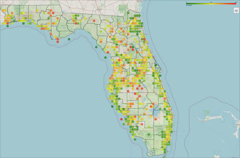
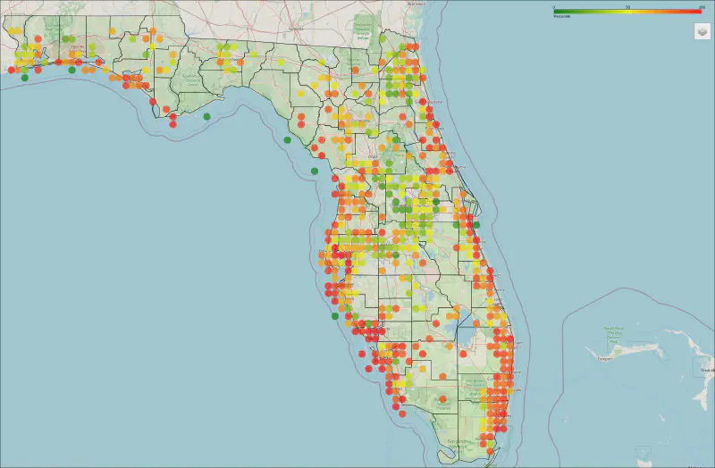
Maps #
The map is interactive and doesn’t embed into my site well (since I use minimal javascript). To view the interactive map, please checkout the cloud notebook. The interactive map has hover-over data.
Otherwise here are a few screenshots of the map:
Energy Burden #
Expected Agricultural Loss due to Natural Hazards Heatmap #
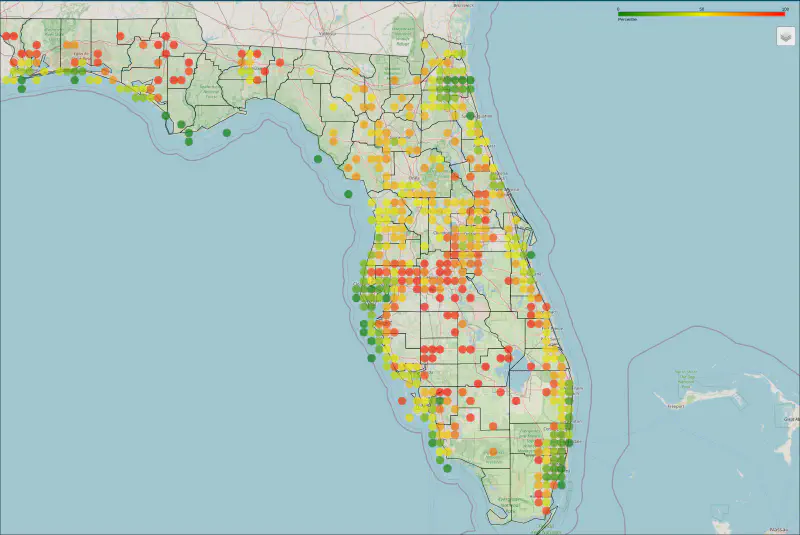
Expected Building Loss due to Natural Hazards Heatmap #
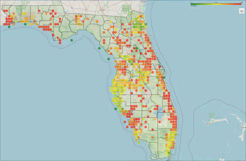
Expected Population Loss due to Natural Hazards Heatmap #
Risk of Fire in 30 years Heatmap #
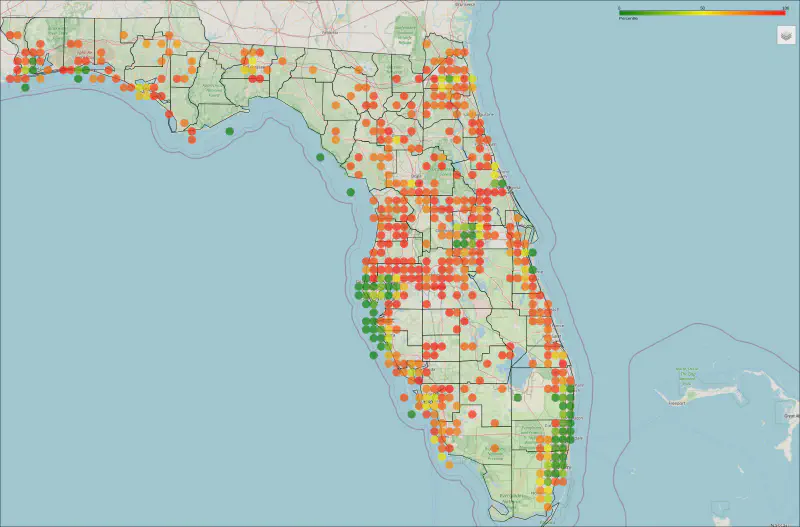
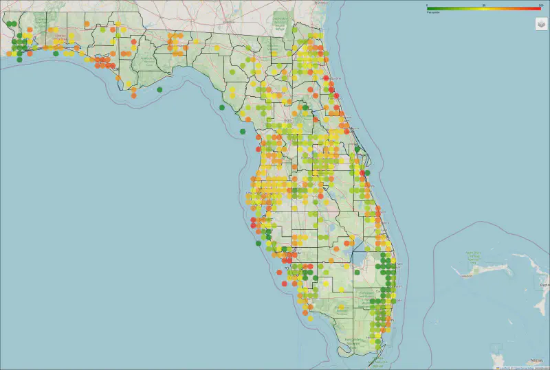
Risk of Flood in 30 years Heatmap #
Continued work: #
Check out the rest of the work the team contributed. If you’d like to continue exploring this data, this was part of challenge 4:
This “getting started” analysis should help answer the following questions
- Where are communities located that have higher vulnerability to natural disasters?
- Who is represented in those communities?
- What is the housing make-up of those communities?
- Analysis insights and questions: What surprised you from this analysis? What are some limitations of the analysis? What are ways to extend the work?
Next steps I’d suggest: Build vulnerability scores
helpful resources: https://eodatascape.datakind.org/